Helmholtz Coil: Complete Guide to Uniform Magnetic Field Generation

Key Takeaways

• Helmholtz coils consist of two identical circular coils separated by a distance equal to their radius, creating a highly uniform magnetic field at the center.
• Named after German physicist Hermann von Helmholtz, they are essential in research requiring precise magnetic field control.

• Configurations can produce uniform fields (Helmholtz) or controlled gradients (Anti-Helmholtz).

• Applications range from canceling Earth’s magnetic field to magnetic moment measurements and biomedical research
• Field strength follows the Biot-Savart law depends on coil radius, turns, current, and permeability of free space.

When experiments demand a precisely defined magnetic environment, researchers turn to the Helmholtz coil—one of the most elegant solutions in electromagnetic engineering. This device generates a nearly uniform field and has become indispensable worldwide, from sensor calibration to quantum physics research.

A Helmholtz coil represents a synergy of theoretical physics and practical engineering. By carefully arranging two identical coils, scientists achieve magnetic fields of predictable uniformity, transforming the way field-dependent measurements are conducted.

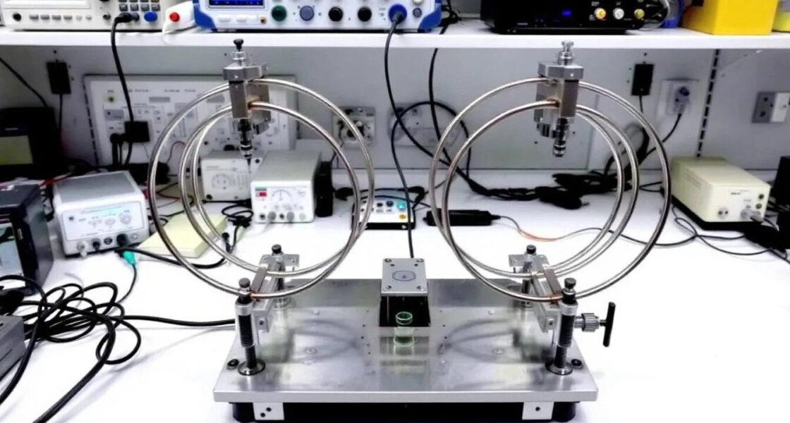
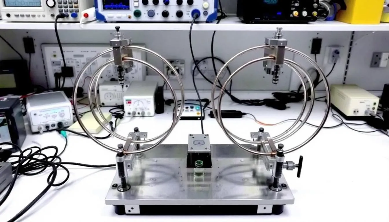
What is a Helmholtz Coil?

A Helmholtz coil consists of two identical circular coils mounted coaxially, carrying equal current in the same direction. The coil spacing equals the radius R, ensuring that their fields combine to form a highly uniform region at the midpoint.

Named after Hermann von Helmholtz, the German physicist who laid the theoretical groundwork in the 19th century, this configuration minimizes spatial field variations and remains the benchmark design for generating controlled magnetic fields.

Key advantage over single coils: while one coil produces a strongly varying field, a Helmholtz pair generates a larger homogeneous zone, critical for precision experiments.

Magnetic Field Theory and Calculations

The coil’s operation is governed by the Biot–Savart law and the principle of superposition. Each coil is modeled as a current loop; the total field is the vector sum of both contributions.

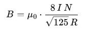
At the center, the field strength is:

Where:

• B represents the magnetic flux density
• μ₀ is the permeability of free space (4π × 10⁻⁷ T⋅m/A)
• N is the number of turns in each coil
• I is the coil current
• R is the radius of the coils

This equation shows direct proportionality: doubling N or $I$ doubles B0​.

Field Along the Axis

• Maximum field occurs at the center point.

• Uniformity extends over a spherical region ≈ 20% of the radius where variation is typically < 1%.

• Taylor expansion analysis explains why: at the center, first- and second-order derivatives vanish, leaving only small higher-order terms.

Real-World Coil Thickness

Practical coils have finite winding cross-sections. The effective coil spacing is measured between midplanes, not edges. Wire bundle geometry, insulation, and winding layout slightly alter the field, so engineering adjustments are required for optimal results.

Variants and Configurations

Square Helmholtz Coils

• Provide larger accessible volume, useful for large specimens or human studies.

• Achieve comparable uniformity but ~5–10% lower field strength than circular coils of equal perimeter.

• Optimal spacing ≈ 0.5445 × side length.

Maxwell Coils (Three-Coil System)

• Three coaxial coils improve uniformity over larger volumes by canceling higher-order field terms.

• Requires carefully maintained radius ratios and ampere-turn ratios.

• Common in materials testing and biological research.

Anti-Helmholtz Coils

• Same geometry, but opposite current in one coil.

• Produces a linear magnetic gradient with zero field at the center.

• Widely used in atomic physics and particle trapping.

Current and Voltage Requirements

DC Operation

• Stable current from a lab power supply ensures accurate static fields.

• Voltage requirement depends on coil resistance (wire gauge, turns, geometry).

• Even small current fluctuations directly cause field variations.

High-Frequency Operation

• Coil inductance increases impedance with frequency.

• At high frequencies, maintaining current requires significantly higher voltage.

• Resonant circuits with capacitors can improve efficiency.

• Limits arise from transmission line effects and eddy currents in nearby conductors.

Applications

Earth’s Field Cancellation

• Helmholtz coils generate a field equal and opposite to Earth’s (≈ 0.25–0.65 gauss), neutralizing interference.

• Full 3D cancellation requires three orthogonal pairs with active feedback control.

3D Field Control

• Three pairs can produce fields in any direction, including rotating or static oriented fields.

• Active compensation stabilizes conditions in noisy environments.

Magnetic Moment Measurements

• Uniform fields enable flux-based measurement of dipole moments.

• Integration with fluxmeters and calibration against standards (e.g., nickel samples) ensures accuracy.

Design Considerations and Optimization

• Spacing: Ideal ≈ radius; slight increase (≈ 1.01 × R) may improve uniformity with little field loss.

• Wire gauge: Thicker wires reduce resistance and heating, allow stronger fields, but affect coil geometry.

• Uniform region: Ensure specimens remain inside homogeneous zone.

• Tolerances: Spacing errors translate into field deviations; precision mechanics are crucial.

• Materials: Support structures must be non-magnetic to avoid distortion.

Calibration and Testing

• Analytical formulas provide estimates, but calibration is essential.

• Tools: Hall sensors and precision magnetometers measure actual field strength.

• Establish a coil constant relating current to field.

• Regular calibration ensures measurement reliability.

• Linearity between input current and output field confirms proper construction.

Frequently Asked Questions (FAQ)

Why is the coil spacing equal to the radius?
This minimizes second-order derivatives of the field at the center, yielding the most uniform possible field for a two-coil setup.

Can Helmholtz coils completely cancel Earth’s field?
Not with a single pair. Full cancellation requires three orthogonal pairs plus feedback control.

What happens if the coil currents are unequal?
Even small differences (~1–2%) reduce uniformity. Series connection ensures identical currents through both coils.

How does wire thickness affect performance?
Thicker wires allow higher current and stronger fields but change coil geometry. Midplane spacing, not edge spacing, must be used.

What limits maximum frequency operation?
Coil inductance, transmission line effects, and eddy currents. Practical limits are typically in the kHz–MHz range.